Supernormal Profit: Perfect and Imperfect Competition
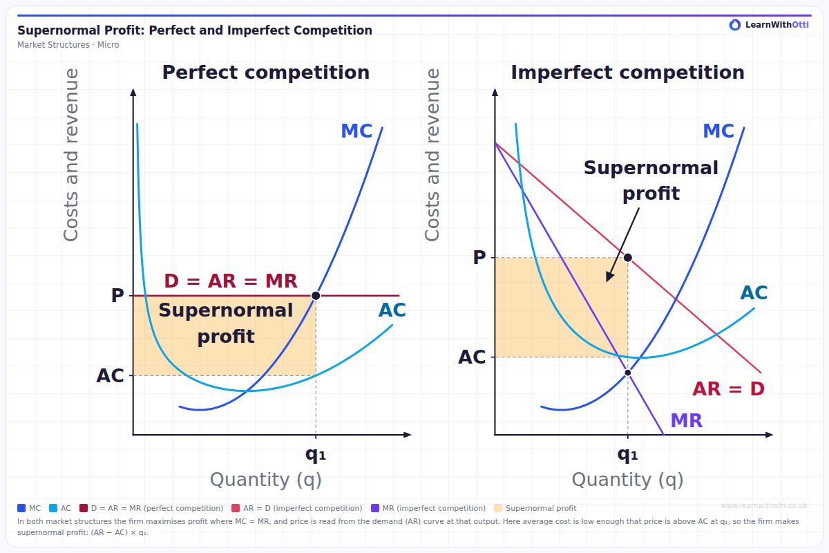
Two-panel diagram comparing a perfectly competitive firm (left) with an imperfectly competitive firm (right), on one price scale and one quantity scale and with the same MC and AC curves. Both produce q₁ where MC = MR on the rising MC, and price is read up from q₁ to the demand (AR) curve. The price taker's demand is horizontal (D = AR = MR); the imperfect competitor's AR slopes down, with MR below it. In both, price is above AC at q₁, so the firm makes supernormal profit, shaded as (AR − AC) × q₁.
Printable preview
Download a static PNG of this diagram to print or include in revision notes.
Download PNGWhat this diagram shows
This is the first of three diagrams in which demand, MR and MC stay exactly the same and only average cost changes. Both firms maximise profit where MC = MR, at q₁ on the rising part of MC, and read the price from their demand (AR) curve at q₁. The price taker's demand curve is horizontal, so D = AR = MR; the imperfect competitor's AR slopes downwards, so its MR lies below AR, with the same intercept and twice the slope. Here fixed costs are low, so AC is low: price is above AC at q₁ and each firm makes supernormal profit, shown by the shaded rectangle (AR − AC) × q₁.
Key points
- Both firms maximise profit where MC = MR, at output q₁ on the rising part of the MC curve.
- The price is read from the AR (demand) curve directly above q₁, not from the point where MC = MR.
- In perfect competition the firm is a price taker, so its demand curve is horizontal and P = AR = MR. In imperfect competition AR slopes downwards and MR lies below it.
- Supernormal profit = (AR − AC) × q₁, using AC at q₁, not the minimum of AC.
- Fixed costs do not affect MC, so they do not change q₁ or the price. Low fixed costs simply give a low AC curve and a large profit rectangle.
Exam tip
Mark q₁ where MC = MR on the rising part of MC, then go up from q₁ to the AR curve to read the price: in imperfect competition the price is on AR, well above the point where MR = MC. Then read AC at the same output. Supernormal profit is (AR − AC) × q₁, the rectangle between the price and AC out to q₁.
Common mistakes
Reading the price at the height where MC = MR in the imperfect competition panel: the firm charges the price on its AR curve above q₁, which is higher. Students also assume that only firms in imperfect competition make supernormal profit, when a price taker can make it in the short run too.
Related diagrams
Normal Profit: Perfect and Imperfect Competition
View →Market StructuresLosses: Perfect and Imperfect Competition
View →Market StructuresProfit Maximisation (MR = MC)
View →Market StructuresPerfect Competition: Short-Run Supernormal Profit
View →Market StructuresMonopoly — Profit Maximisation
View →Ask Otti about this diagram
Our AI tutor can walk you through every curve, explain exam technique, and quiz you on it.