AQA A-Level Economics · Revision notes
4.1.4.5 Economies and Diseconomies of Scale
As a firm grows, its average costs change. Up to a point, producing on a larger scale makes each unit cheaper to make. Beyond that point, size can start to raise costs. These two effects, economies and diseconomies of scale, explain the shape of the long-run average cost curve, including the L-shaped curve and the minimum efficient scale.
Economies of scale
Economies of scale are the reductions in long-run average cost that come from increasing the scale of production. On a diagram, they appear as the falling part of the LRAC curve.
Internal and external economies of scale
Internal economies of scale come from the growth of the individual firm. They move the firm along its LRAC curve.
Key distinction: External economies of scale come from the growth of the industry as a whole, often in a particular area. They benefit all firms in the industry and shift the LRAC curve downwards.
Examples of external economies:
- a pool of skilled labour concentrated in an area;
- specialist suppliers and services locating nearby;
- shared infrastructure such as transport links;
- local training and research institutions serving the industry.
Clusters such as financial services in the City of London or technology firms in Cambridge benefit from these effects.
External diseconomies of scale can also arise when an industry grows too large in one area, for example through congestion, competition for scarce skilled labour, or rising land prices. These shift the LRAC curve upwards.
Types of internal economies of scale
Internal economies arise from the growth of the firm itself.
Technical economies
- Larger firms can use larger, more efficient machinery that would not be worthwhile at small output.
- Some costs rise less than proportionately with capacity. A container ship twice as large does not need twice the crew or twice the fuel.
- Large firms can spread the fixed cost of equipment, and of research, over more units.
Purchasing economies Buying inputs in bulk allows firms to negotiate lower prices from suppliers. Large supermarket chains are the classic example.
Marketing economies The cost of an advertising campaign can be spread across a much larger output, so the advertising cost per unit falls.
Managerial economies Large firms can employ specialist managers for finance, marketing and human resources, who work more efficiently than a few generalists.
Financial economies Large firms are seen as less risky by lenders, so they can borrow more easily and at lower interest rates. They can also raise funds by issuing shares.
Risk-bearing economies Large firms can diversify across products and markets, so a fall in demand in one area does less damage to the business as a whole.
Diseconomies of scale
Diseconomies of scale are increases in long-run average cost as a firm grows beyond a certain size. They appear as the rising part of the LRAC curve.
They come mainly from the difficulty of managing a very large organisation:
- Communication problems. More layers of management slow down the flow of information, and messages become distorted.
- Coordination problems. It becomes harder to make sure every part of the firm works towards the same goals.
- Control problems. Senior managers find it harder to monitor what is happening across the business, and inefficiency can go unnoticed.
- Motivation problems. Workers in very large organisations may feel remote from decisions and less valued, reducing effort and raising absence.
Returns to scale and economies of scale
Returns to scale describe what happens to output when a firm increases all of its inputs in the same proportion. As long as factor prices do not change, they link directly to long-run average cost.
- Increasing returns to scale: output rises by a larger percentage than inputs, so cost per unit falls. This is a source of economies of scale.
- Constant returns to scale: output rises by the same percentage as inputs, so long-run average cost stays the same.
- Decreasing returns to scale: output rises by a smaller percentage than inputs, so cost per unit rises. This is a source of diseconomies of scale.
Economies of scale are a wider idea, because they also include savings such as cheaper bulk buying or cheaper finance.
Minimum efficient scale
Minimum efficient scale (MES) is the lowest level of output at which long-run average cost is minimised. It is the point where the LRAC curve first reaches its lowest level.
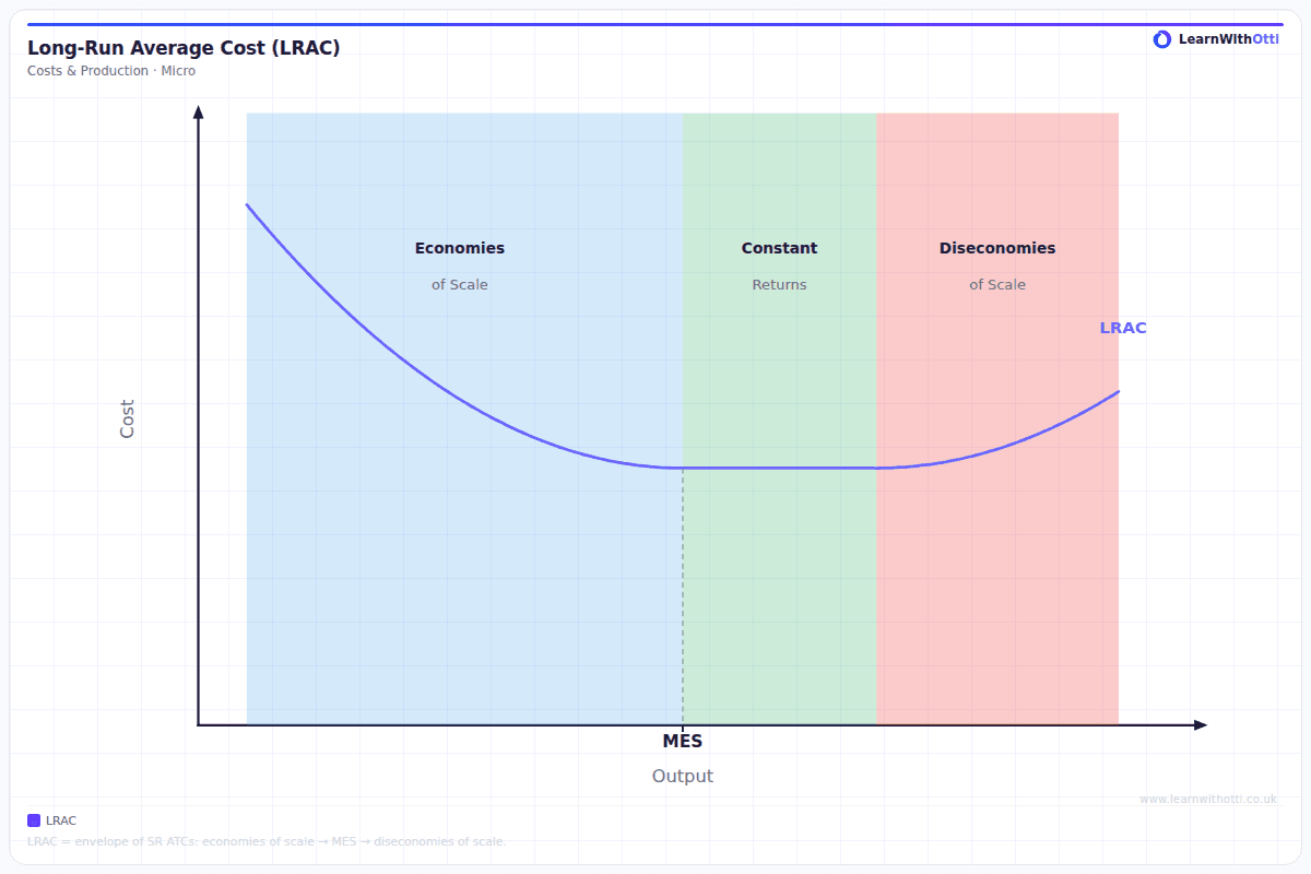
MES matters for the structure of an industry:
- If MES is low relative to market demand, many firms can operate at lowest cost, so the market can support plenty of competitors.
- If MES is high relative to market demand, only a few firms can achieve lowest cost. The market tends towards oligopoly.
- If MES is so high that one firm can supply the whole market at lower cost than two or more could, the market is a natural monopoly. Water supply and rail networks are typical examples.
Key idea: The low average costs that established firms reach at the MES act as a barrier to entry: a new entrant starting at a small scale cannot match those costs, so it struggles to compete on price.
The L-shaped long-run average cost curve
In the long run, a firm can change all its inputs, including the size of its factory. Each possible scale of plant has its own short-run average cost (SRAC) curve.
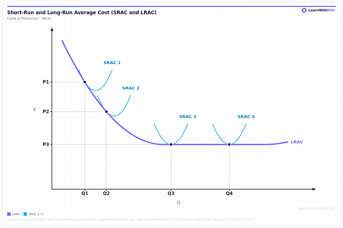
Each SRAC in the diagram represents a different size of plant. A firm producing Q1 with the plant of SRAC 1 has an average cost of P1. Moving to the larger plant of SRAC 2 lowers average cost to P2 at Q2, and the plant of SRAC 3 lowers it again to P3 at Q3. These falls in average cost as the firm grows are economies of scale. Between Q3 and Q4 average cost stays at P3, so a still larger plant brings no further saving. This is constant returns to scale.
Key distinction: The LRAC is often drawn U-shaped, falling and then rising. It can also fall and then flatten out, as in the diagram, when beyond a certain size growth brings neither further savings nor extra costs. Either way, its shape comes from economies and diseconomies of scale, not from diminishing returns, which apply only in the short run.
A curve that falls and then stays flat over a wide range of output is called an L-shaped LRAC. Many economists argue it is closer to reality than the U shape, because large firms can often avoid diseconomies of scale, for example by splitting into smaller divisions. Minimum efficient scale marks the start of the flat section.
Key terms
| Term | Meaning |
|---|---|
| Economies of scale | Falling long-run average cost as the scale of production increases |
| Diseconomies of scale | Rising long-run average cost as a firm grows beyond a certain size |
| Internal economies | Cost savings from the growth of the firm itself |
| External economies | Cost savings from the growth of the industry, shared by all its firms |
| Returns to scale | The change in output when all inputs are increased in the same proportion |
| Minimum efficient scale | The lowest output at which long-run average cost is minimised |
| L-shaped LRAC | A long-run average cost curve that falls and then stays flat beyond minimum efficient scale |
| Natural monopoly | A market where one firm can supply total demand at lower cost than several firms |
Common mistakes
- Confusing economies of scale with diminishing returns. Diminishing returns are a short-run idea with a fixed factor; economies of scale are long run, with all factors variable.
- Moving along the LRAC curve for an external economy. External economies shift the whole curve down.
- Explaining diseconomies with lost economies. Diseconomies are rising costs from managing size, not the absence of savings.
- Defining MES as the lowest point of a short-run curve. It refers to the long-run average cost curve.
- Listing types without explaining why unit cost falls. Each type needs a mechanism: spreading a fixed cost, a lower price per unit, or cheaper finance.
How this has been examined
In the AQA papers indexed on this site, this topic has appeared in three formats:
- 15-mark "Explain" essay — asked twice across 2 series (2021 to 2024)
- 9-mark "Explain" data response — asked twice across 2 series (2019 to 2025)
- 1-mark multiple choice — asked once (2018)
Where this goes next
The long-run average cost curve that these economies shape is introduced in 4.1.4.4 Costs of production, and returns to scale in 4.1.4.3 The law of diminishing returns and returns to scale. High minimum efficient scale explains the natural monopoly case in 4.1.5.6 Monopoly and monopoly power and acts as a barrier to entry in 4.1.5.9 Contestable and non-contestable markets. Producing at the lowest point of the average cost curve is the condition for productive efficiency in 4.1.5.10 Market structure, static efficiency, dynamic efficiency and resource allocation.
Otti is an AI tutor built for A-Level students. Ask it anything, practise exam questions, and get instant feedback written like an examiner would give it — not just right or wrong, but why.
Get one answer marked free