AQA A-Level Economics · Revision notes
4.1.5.11 Consumer and Producer Surplus
When you buy a coffee for £3 that you would happily have paid £5 for, you have gained £2 of value that never appears in any transaction record. Economists call that consumer surplus, and it is how the welfare generated by a market is measured. This page covers how to show consumer and producer surplus on a diagram, how they change when demand and supply shift, and how to use them to analyse monopoly and price discrimination.
Consumer surplus
Consumer surplus is the difference between what consumers are willing to pay and what they actually pay.
The demand curve shows willingness to pay. The first unit is bought by someone valuing it highly; later units by people valuing it less. But everyone pays the same market price.
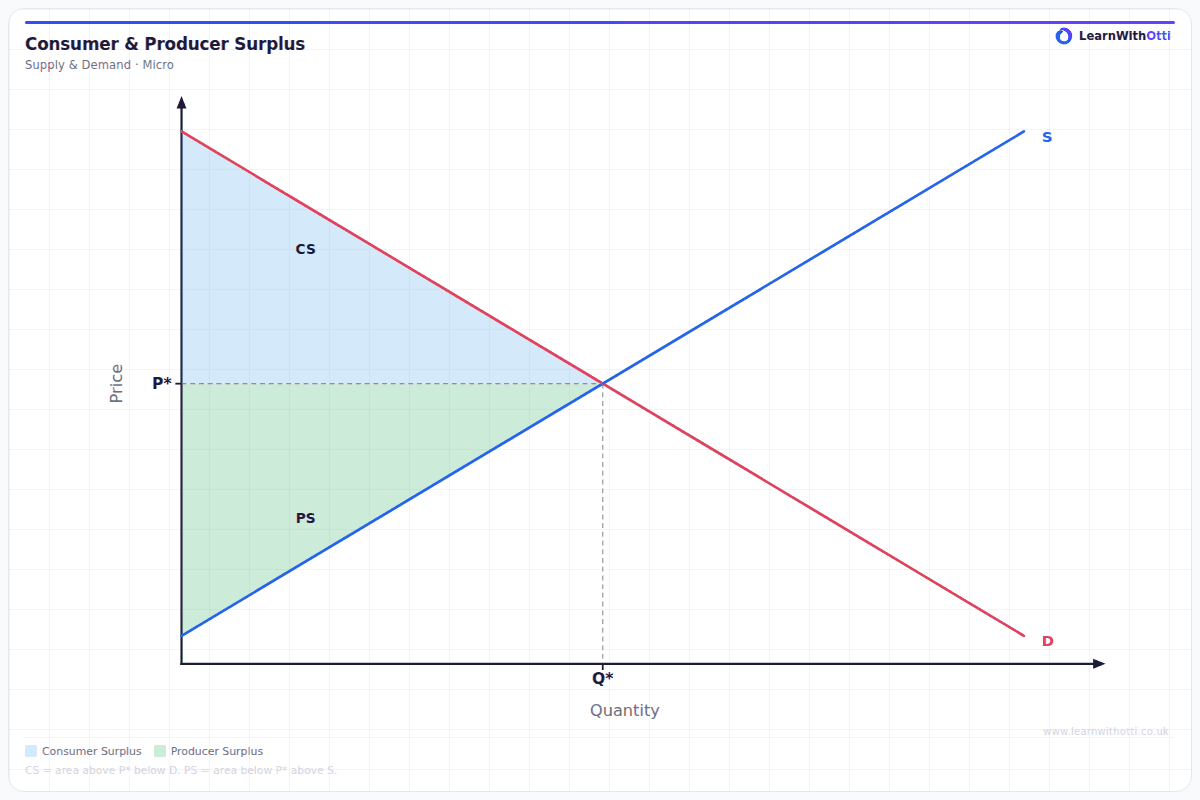
On a diagram, consumer surplus is the area below the demand curve and above the price, up to the quantity traded.
Producer surplus
Producer surplus is the difference between the price producers receive and the minimum they would have accepted.
The supply curve shows the minimum acceptable price for each unit, reflecting the cost of producing it. The first units are cheap to produce; later units cost more. But every unit sells at the same market price.
On a diagram, producer surplus is the area above the supply curve and below the price, up to the quantity traded.
Total welfare
Total welfare (or community surplus) = consumer surplus + producer surplus.
It is the triangle between the two curves, up to the equilibrium quantity.
Key idea: At the free-market equilibrium in a market without failure, this area is at its maximum, which illustrates why competitive markets are efficient.
Any intervention or distortion that moves the market away from equilibrium reduces total welfare, and the loss is called deadweight loss. That is the analytical tool underlying almost every intervention question later in the course.
How changes in demand and supply affect surplus
An increase in demand (shift right) raises price and quantity.
- Producer surplus rises, unambiguously: higher price and more units sold.
- Consumer surplus is ambiguous. Consumers pay more per unit, which reduces it, but more units are bought and new consumers enter the market. The net effect depends on elasticity.
An increase in supply (shift right) lowers price and raises quantity.
- Consumer surplus rises, unambiguously: lower price and more units.
- Producer surplus is ambiguous: lower price per unit but more units sold.
A decrease in either curve reverses these.
The useful generalisation: a shift in one curve unambiguously benefits the other side of the market, while the effect on the side that shifted depends on the relative size of the price and quantity changes — which is an elasticity question.
Elasticity and the size of the surplus
- The more inelastic demand is, the larger consumer surplus tends to be, because consumers were willing to pay much more than they do.
- The more inelastic supply is, the larger producer surplus tends to be.
- At the extremes: with perfectly elastic demand there is no consumer surplus at all, since consumers pay exactly what they were willing to pay.
Where surplus analysis is used
This is not an abstract exercise. Consumer and producer surplus is the measuring tool for:
- Indirect taxes, where the tax transfers surplus to the government and destroys some entirely as deadweight loss.
- Subsidies, which raise both surpluses at a cost to taxpayers.
- Price controls: a maximum price raises consumer surplus for those who can still buy, but creates a shortage and a deadweight loss.
- Monopoly, where restricted output transfers consumer surplus to the producer and creates deadweight loss.
- Tariffs, where the same analysis applies internationally.
Monopoly and deadweight loss
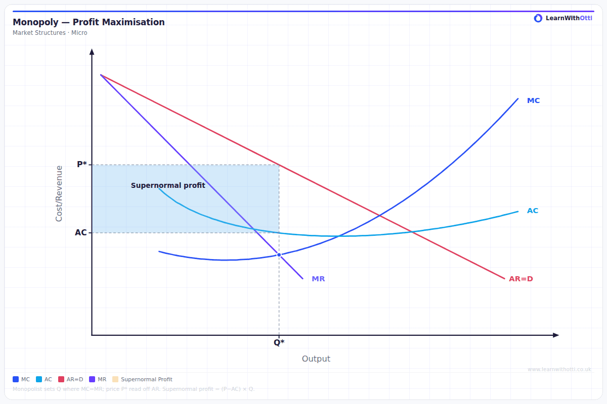
The monopoly diagram shows AR and MR sloping downwards, with MC and AC curves. Compared with a competitive market with the same costs:
- Output is lower and price is higher. A competitive market would produce where price equals MC; the monopolist restricts output to where MC = MR.
- Not allocatively efficient, because price is above MC.
- Deadweight welfare loss. The units between the monopoly output and the competitive output would have been worth more to consumers than they cost to produce, but are not produced. This lost welfare is a triangle between the demand curve and MC.
In surplus terms, part of the consumer surplus becomes producer surplus, because consumers pay a higher price on the units they still buy. The rest of the lost consumer surplus is not gained by anyone. It is the deadweight loss.
Price discrimination and surplus
Price discrimination is charging different prices to different groups of customers for the same product, where the price difference does not reflect any difference in cost. Third-degree price discrimination divides customers into separate groups, such as peak and off-peak rail travellers, or adults and students at the cinema.
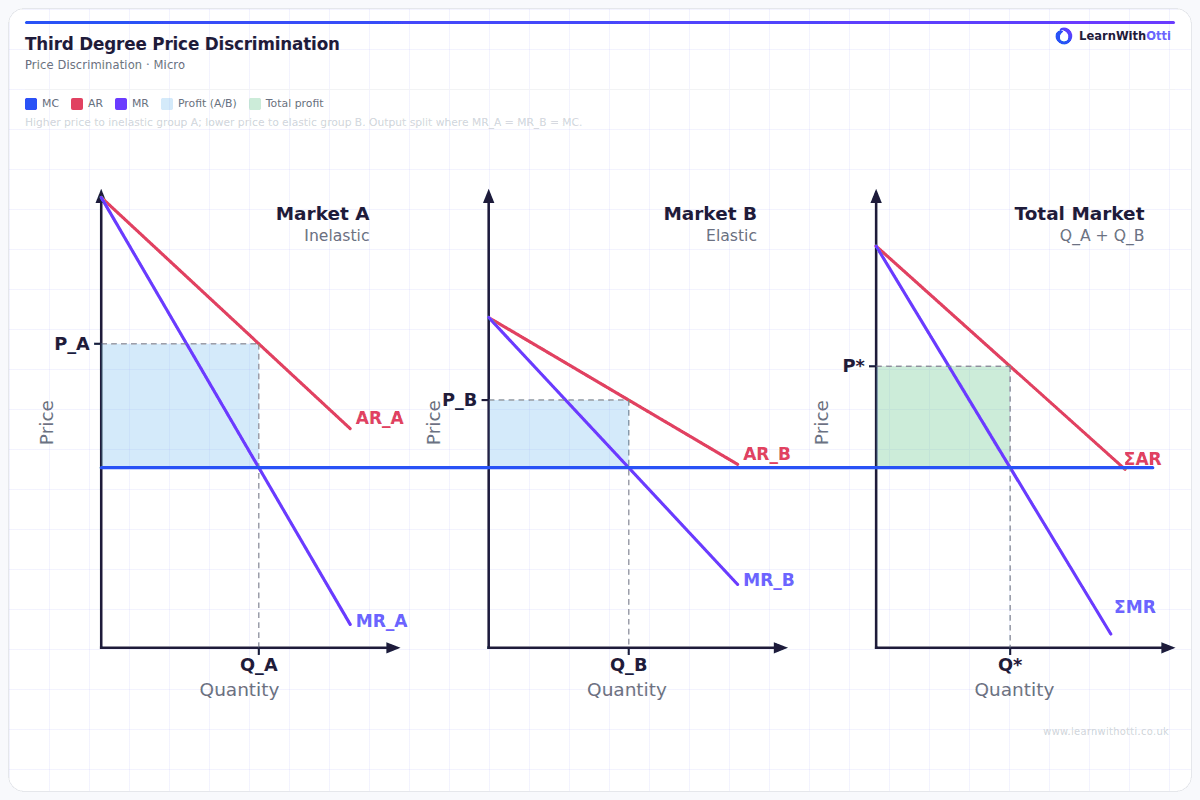
Costs and benefits:
- Producers gain higher profits, which may fund investment.
- Consumers with inelastic demand lose: they pay more, and some of their consumer surplus becomes producer surplus.
- Consumers with elastic demand may gain: some people, such as students or off-peak travellers, can buy a product they could not otherwise afford.
- Output may rise overall, which can make a service viable that would not run at a single price, such as a rail service that is profitable only with both peak and off-peak fares.
In the extreme case of first-degree (perfect) price discrimination, every consumer pays the maximum they are willing to pay. All consumer surplus becomes producer surplus. Output rises to the competitive level, where price equals marginal cost, so there is no deadweight loss, but consumers as a group are worse off.
Key terms
| Term | Meaning |
|---|---|
| Consumer surplus | The difference between willingness to pay and the price actually paid |
| Producer surplus | The difference between the price received and the minimum acceptable |
| Total welfare | Consumer surplus plus producer surplus; also community surplus |
| Deadweight loss | Welfare lost when a market produces away from the efficient quantity |
| Willingness to pay | The maximum a consumer would pay, shown by the demand curve |
| Third-degree price discrimination | Charging different prices to separate groups of customers for the same product |
| First-degree price discrimination | Charging each consumer the maximum they are willing to pay, so no consumer surplus remains |
Common mistakes
- Getting the areas the wrong way round. Consumer surplus is above the price and below demand; producer surplus is below the price and above supply. Remember that consumers benefit from a low price, so their area sits above it.
- Measuring surplus beyond the quantity traded. Both areas stop at the equilibrium quantity. Units never produced generate no surplus.
- Saying an increase in demand raises consumer surplus. It is ambiguous: price rises, which works against consumers, even as more units are bought.
- Confusing producer surplus with profit. Producer surplus is revenue minus variable cost; it does not account for fixed costs, so it is not the same as profit.
- Drawing the areas without labelling them. The diagram only communicates if the regions are shaded and named.
- Charging the higher price in the elastic market. The higher price goes to the group with inelastic demand.
How this has been examined
In the AQA papers indexed on this site, this topic has appeared in two formats:
- 15-mark "Explain" essay — asked twice across 2 series (2020 to 2024)
- 1-mark multiple choice — asked twice across 2 series (2022 to 2025)
Where this goes next
The equilibrium these areas are measured from is set in 4.1.3.5 The determination of equilibrium market prices, and the efficiency argument the surplus maximum supports is developed in 4.1.8.1 How markets and prices allocate resources. The monopoly and price discrimination analysis is covered in full in 4.1.5.6 Monopoly and monopoly power and 4.1.5.7 Price discrimination, and efficiency across market structures in 4.1.5.10 Market structure, static efficiency, dynamic efficiency and resource allocation. Surplus is the measuring tool for taxes, subsidies and price controls in 4.1.8.9 Government intervention in markets.
End of topic 4.1.5
Quiz yourself on 4.1.5 Perfect competition, imperfectly competitive markets and monopoly
10 multiple-choice questions drawn from the 21 we have on the whole of topic 4.1.5, with instant feedback on every answer.
Start the 4.1.5 quiz →Otti is an AI tutor built for A-Level students. Ask it anything, practise exam questions, and get instant feedback written like an examiner would give it — not just right or wrong, but why.
Get one answer marked free