Edexcel A-Level Economics · Revision notes
3.3.2 Costs
Costs are the other half of the profit calculation. This topic covers the main cost measures, why short-run cost curves have the shapes they do, and how short-run and long-run average costs relate.
Fixed and variable costs
The short run is a period in which at least one factor of production is fixed, usually capital. In the long run, all factors are variable.
- Fixed costs do not change with output in the short run. Examples include rent, insurance and interest on loans. They must be paid even if output is zero.
- Variable costs change directly with output. Examples include raw materials, energy used in production and wages of hourly staff.
The cost formulae
| Measure | Formula |
|---|---|
| Total cost (TC) | TC = TFC + TVC |
| Total fixed cost (TFC) | Constant at every output in the short run |
| Total variable cost (TVC) | Rises with output |
| Average (total) cost (AC) | AC = TC / Q, also AFC + AVC |
| Average fixed cost (AFC) | AFC = TFC / Q |
| Average variable cost (AVC) | AVC = TVC / Q |
| Marginal cost (MC) | MC = change in TC / change in Q |
Watch out: Because fixed costs do not change with output, marginal cost depends only on changes in variable cost.
A worked example
A firm has fixed costs of £100.
| Q | TFC | TVC | TC | AFC | AVC | AC | MC |
|---|---|---|---|---|---|---|---|
| 0 | 100 | 0 | 100 | — | — | — | — |
| 1 | 100 | 50 | 150 | 100 | 50 | 150 | 50 |
| 2 | 100 | 90 | 190 | 50 | 45 | 95 | 40 |
| 3 | 100 | 120 | 220 | 33.3 | 40 | 73.3 | 30 |
| 4 | 100 | 160 | 260 | 25 | 40 | 65 | 40 |
| 5 | 100 | 220 | 320 | 20 | 44 | 64 | 60 |
| 6 | 100 | 300 | 400 | 16.7 | 50 | 66.7 | 80 |
AFC falls continuously as fixed cost is spread over more units. MC first falls and then rises. AVC and AC fall and then rise, and MC rises through each of them close to their minimum points.
Why short-run cost curves are shaped as they are
The shapes come from the law of diminishing marginal productivity (diminishing marginal returns).
In the short run, a firm adds more of a variable factor, such as labour, to a fixed factor, such as a factory.
- At first, extra workers allow specialisation and better use of the fixed capital, so each additional worker adds more output than the last. Marginal productivity rises, and MC falls.
- Eventually, the fixed factor becomes crowded. Each additional worker adds less output than the previous one. Marginal productivity falls, so each extra unit of output needs more labour, and MC rises.
This produces:
- a U-shaped MC curve, falling then rising;
- U-shaped AVC and AC curves, falling while MC is below them and rising once MC is above them;
- a continuously falling AFC curve.
Why MC cuts AVC and AC at their minimum points This is arithmetic.
Key idea: If the cost of the next unit is below the average, it pulls the average down. If it is above the average, it pulls the average up. So the average falls while MC is below it and rises once MC is above it, which means MC must cross the average at its lowest point.
The gap between AC and AVC is AFC, which narrows as output rises.
Short-run and long-run average cost curves
In the long run, a firm can change all its inputs, including the size of its factory. Each possible scale of plant has its own short-run average cost (SRAC) curve.
The long-run average cost (LRAC) curve shows the lowest possible average cost of producing each output when the firm can choose any scale of plant. It is drawn as an envelope around the SRAC curves, touching each one.
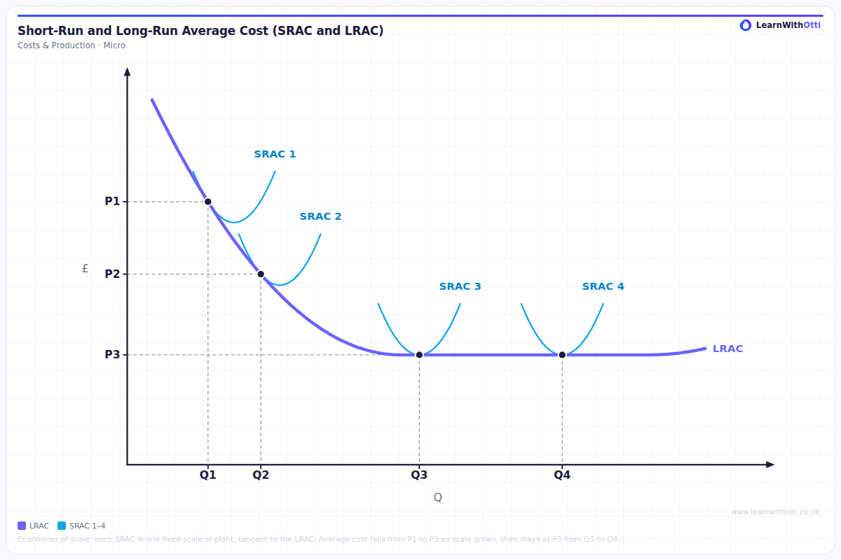
Each SRAC in the diagram represents a different size of plant. A firm producing Q1 with the plant of SRAC 1 has an average cost of P1. Moving to the larger plant of SRAC 2 lowers average cost to P2 at Q2, and the plant of SRAC 3 lowers it again to P3 at Q3. These falls in average cost as the firm grows are economies of scale. Between Q3 and Q4 average cost stays at P3, so a still larger plant brings no further saving. This is constant returns to scale.
- The LRAC can never be above an SRAC, because in the long run the firm can always choose the plant size that gives the lowest cost.
Key distinction: The LRAC is often drawn U-shaped, falling and then rising. It can also fall and then flatten out, as in the diagram, when beyond a certain size growth brings neither further savings nor extra costs. Either way, its shape comes from economies and diseconomies of scale, not from diminishing returns, which apply only in the short run.
Key terms
| Term | Meaning |
|---|---|
| Short run | A period in which at least one factor of production is fixed |
| Long run | A period in which all factors of production are variable |
| Fixed cost | A cost that does not vary with output in the short run |
| Variable cost | A cost that varies directly with output |
| Marginal cost | The change in total cost from producing one more unit |
| Diminishing marginal productivity | Each extra unit of a variable factor adds less output than the previous one, once the fixed factor is fully used |
| LRAC | The lowest average cost of each output when all inputs can vary |
Common mistakes
- Explaining the U-shaped LRAC with diminishing returns. Diminishing returns are a short-run idea; LRAC's shape comes from economies and diseconomies of scale.
- Drawing MC crossing AC away from its minimum. MC must pass through the lowest points of AVC and AC.
- Including fixed costs in marginal cost. Fixed costs do not change with output, so they never affect MC.
- Drawing AFC as U-shaped. AFC falls continuously.
- Treating the short run as a fixed length of time. It is defined by whether any factor is fixed, which varies between industries.
How this has been examined
In the Edexcel papers indexed on this site, this topic has appeared in six formats:
- 1-mark multiple choice — asked twice across 2 series (2017 to 2020)
- 2-mark calculation — asked once (2020)
- 2-mark "Explain" data response — asked once (2020)
- 2-mark "Explain" short answer — asked once (2017)
- 5-mark "Explain" data response — asked once (2021)
- 25-mark "Evaluate" essay — asked once (2024)
Where this goes next
The economies and diseconomies that shape the LRAC curve are covered in 3.3.3 Economies and diseconomies of scale. Costs are combined with revenue from 3.3.1 Revenue to identify profit and shut-down points in 3.3.4 Normal profits, supernormal profits and losses, and the lowest point of the AC curve defines productive efficiency in 3.4.1 Efficiency.
Otti is an AI tutor built for A-Level students. Ask it anything, practise exam questions, and get instant feedback written like an examiner would give it — not just right or wrong, but why.
Get one answer marked free